Quest for autism biomarkers faces steep statistical challenges

Every week, scientists publish new studies reporting differences between people with and without autism. Many of these studies involve some form of biological test — for example, a brain scan, a blood test or a measure of eye movements.

Coverage of these studies in academia and the popular media often suggests that the test in question could serve as a ‘biomarker’ for autism — an objective way of determining whether someone has the condition. The hope is that biomarkers could one day allow clinicians to identify people with autism earlier, more accurately and more efficiently than is currently possible.

These are noble objectives. But with any potential biomarker, finding a difference, on average, between people with and without autism is only the first small step toward clinical utility.

When it comes to diagnosis, clinicians don’t care about group averages. No test is perfect, but for a biomarker to be useful, clinicians need to be able to look at the test results of an individual and determine with some degree of confidence whether that person has autism.

Our aim in this article is to explain some of the key statistics that scientists use to determine just how useful and accurate a test is — in both the lab and the clinic.

Making the cut:

The first point to note is that most tests produce a range or distribution of scores across the population (see graphic below). Even if the distributions differ for people with and without autism, there is almost always some overlap between the two groups. The best we can do is set a cutoff and say that anyone scoring above the cutoff has tested positive.

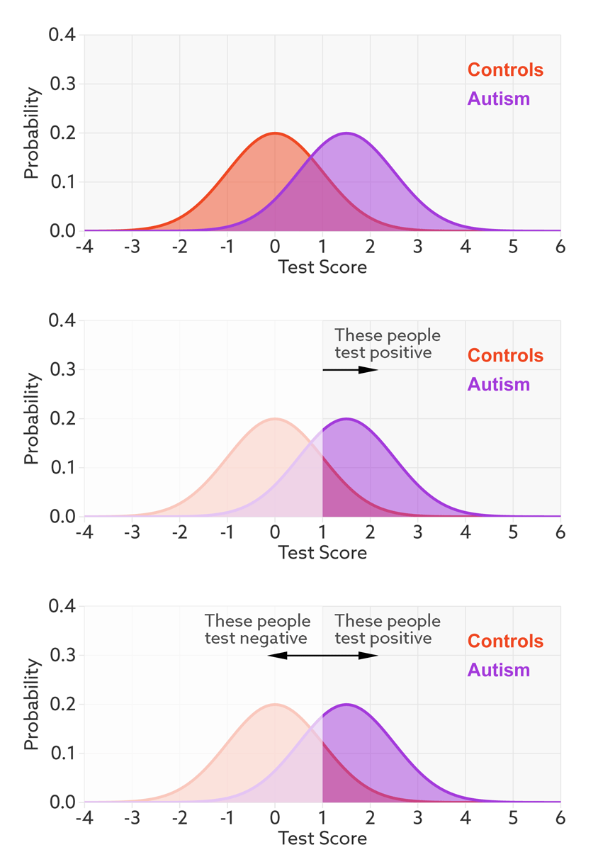
Having set a cutoff, researchers can quantify the accuracy of the test in terms of its ‘sensitivity’ and rate of false positives. Sensitivity refers to the proportion of people with autism who are correctly identified as having autism. The false-positive rate is the proportion of people without autism who are incorrectly identified as having the condition. (Sometimes researchers report the ‘specificity’ or ‘true negatives’ of the test instead of the false-positive rate.)

The sensitivity and false-positive rate both depend on the chosen cutoff. If we lower the cutoff score for autism, more people with the condition test positive and the sensitivity increases (see graphic below). But this also means capturing more people who don’t have autism, thereby increasing the rate of false positives.

Research papers typically represent this trade-off by plotting the test’s ‘receiver operating characteristic (ROC).’ This shows the sensitivity of a test plotted against its false-positive rate for each possible cutoff score.

ROC curves tell us how well a test discriminates between people with and without autism. The less overlap there is between the two distributions, the better the test discriminates between the two groups, and the more the ROC arches above the diagonal (see graphic below).

True diagnosis:

Many scientific reports stop at this point. It’s tempting to assume that a strongly arched ROC means that the test could serve as a helpful diagnostic.

The trouble, however, is that the sensitivity and false-positive rate really only make sense in a context where we know from the outset who has autism and who doesn’t. Sensitivity, for example, tells us how well the test identifies people we already know to have autism.

In real-life scenarios, we don’t usually know the person’s true diagnosis beforehand — that’s the whole reason for administering the test.

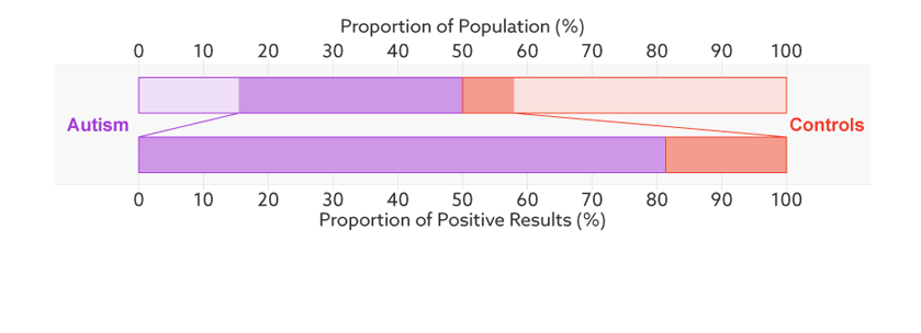
Consider, for example, a parent whose child has just tested positive for autism. What they really need to know is the likelihood that their child actually has autism. We refer to this as the test’s ‘positive predictive value’ — the likelihood that a positive test result is accurate (see bar graph).

Base rates:

There’s one final complication. Unlike the sensitivity or false-positive rate, the positive predictive value depends on the proportion of people being tested who truly have autism. We refer to this as the sample’s autism ‘base rate.’

In a typical study, the base rate is around 50 percent: People with autism make up half the sample. But in many contexts outside the lab, the base rate is much lower: Most people taking the test won’t have autism.

Say that our hypothetical biomarker is being used to screen all children in a particular age range for autism. According to the latest estimate from the U.S. Centers for Disease Control and Prevention, the prevalence of autism in the United States among school-age children is about 1 in 68. Clinicians could therefore expect to test roughly 67 children who don’t have autism for every one child who does.

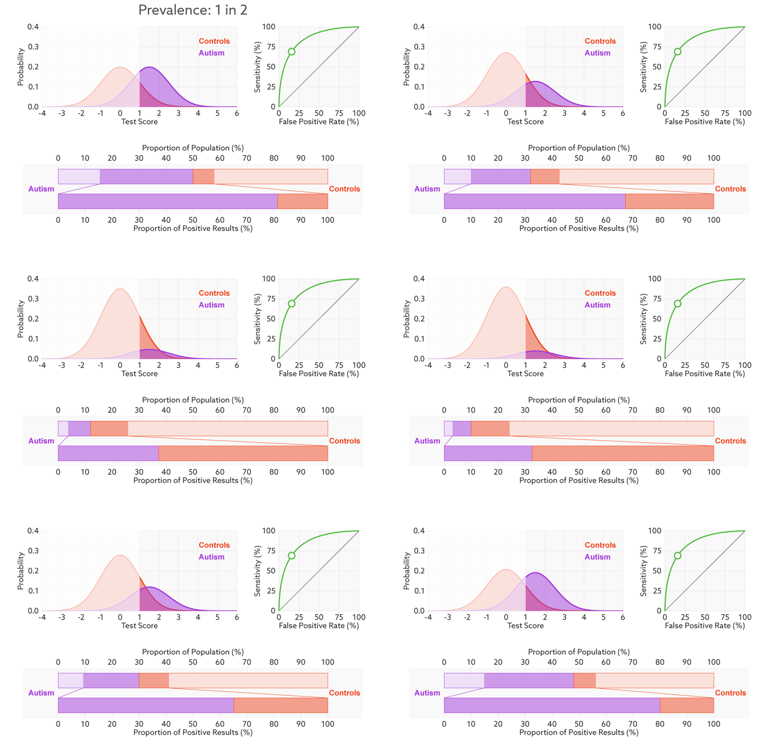
Changing the base rate from 1 in 2 (50 percent) to 1 in 68 (1.5 percent) has a dramatic effect on the positive predictive value. In our fictitious example (see graphic below), it falls from 81 percent to a much less helpful 6 percent. In other words, for every 6 children the test correctly identifies, it would misidentify 94 children as having autism who don’t.

In the context of population screening, a positive result would only indicate an increased risk of having autism. Clinicians would need to follow up with further tests to confirm a diagnosis.

Until such assessments are completed, ‘autism risk’ is nothing more than the test’s positive predictive value. The base rate issue means that most children flagged as ‘at risk’ will not actually have autism.

So although early identification has potential benefits, an ‘at risk’ label may also cause unnecessary stress to large numbers of families. In some cases, children may receive intervention for autism that isn’t present, diverting resources away from children who genuinely have the condition.

Difficult distinctions:

An alternative to population screening is to target groups in which the autism base rate is already higher than that of the general population — for example, children who have an older sibling with autism, or those whose parents or doctors are concerned about their development. This approach makes a lot of sense. But we can’t simply adjust the base rate in our calculations and assume that the test retains the same sensitivity and false-positive rate.

Consider, for example, a hypothetical test that identifies genetic variations associated with autism. These variations may also be relatively common in the siblings of individuals with autism. So even if the genetic test discriminates well between people with autism and unrelated individuals, it may do a much poorer job of differentiating between affected and unaffected members of the same family.

Researchers would need to conduct a new study to determine how well the test performs in this high-risk population.

At present, autism diagnosis is a difficult, time-consuming and resource-intensive affair. Early signs are often missed and, even when recognized, children can wait years for a formal diagnosis. Adults may struggle their entire lives without anyone recognizing the difficulties they face.

It is important then for researchers to continue developing better ways of identifying and diagnosing people with autism. But when considering potential autism biomarkers, it’s also important to be aware of the challenges inherent in translating an exciting research finding into a test that is clinically useful.

Moving the mark:

Move the sliders to see the effects of changing a hypothetical test’s effect size (a measure of how well it discriminates between groups), the prevalence of autism in the population (base rate), and the cutoff for a positive test.

*Technical note: For illustrative purposes, our figures assume that test scores have normal distributions with equal variance for the two groups (people with and without autism). Test score is represented as the number of standard deviations from the average of the control group. The effect size is then equivalent to the difference of the averages.